Big O Notation

What is Big O?

Big O is a measure of the efficiency of an algorithm as its input size increases. Big O efficiency is measured in terms of time or space requirements. Big O efficiency is based on the number of items (usually indicated by n). Big O measures growth of a function as arguments approach infinity (scale vs speed). Big O notation is also known as asymptotic notation.

Big O notation approximates the growth rate of a function. Big O notation does not give exact measurement of runtime or resource usage. The Big O notation complexity measure is independent of hardware or implementation details.

Platform independence means we don't consider:

Hardware
Operating System
CPU
Arithmetic Precision
Programming Language
Compiler/Interpreter quality
Network factors

All these will definitely affect the performance of an algorithm but Big O will not take this into consideration. Sorting 1000 numbers could take less than a second in today's computers, but computers from 30 or 40 years ago may take a few seconds or a couple of minutes to sort them. Does that mean that the algorithm from the past is less effective? That's not the case. We may be using the same exact algorithm, but the way we measure efficiency we will not have to look at the hardware.

Pronunciation

Big O notation can be read in multiple ways

Big oh of n
Order of n
Oh of n

Big O Notation Complexity

Complexity	Name
	constant
	logarithmic
	linear
	linearithmic
	quadratic
	cubic
	exponential
	factorial

Growth Rates

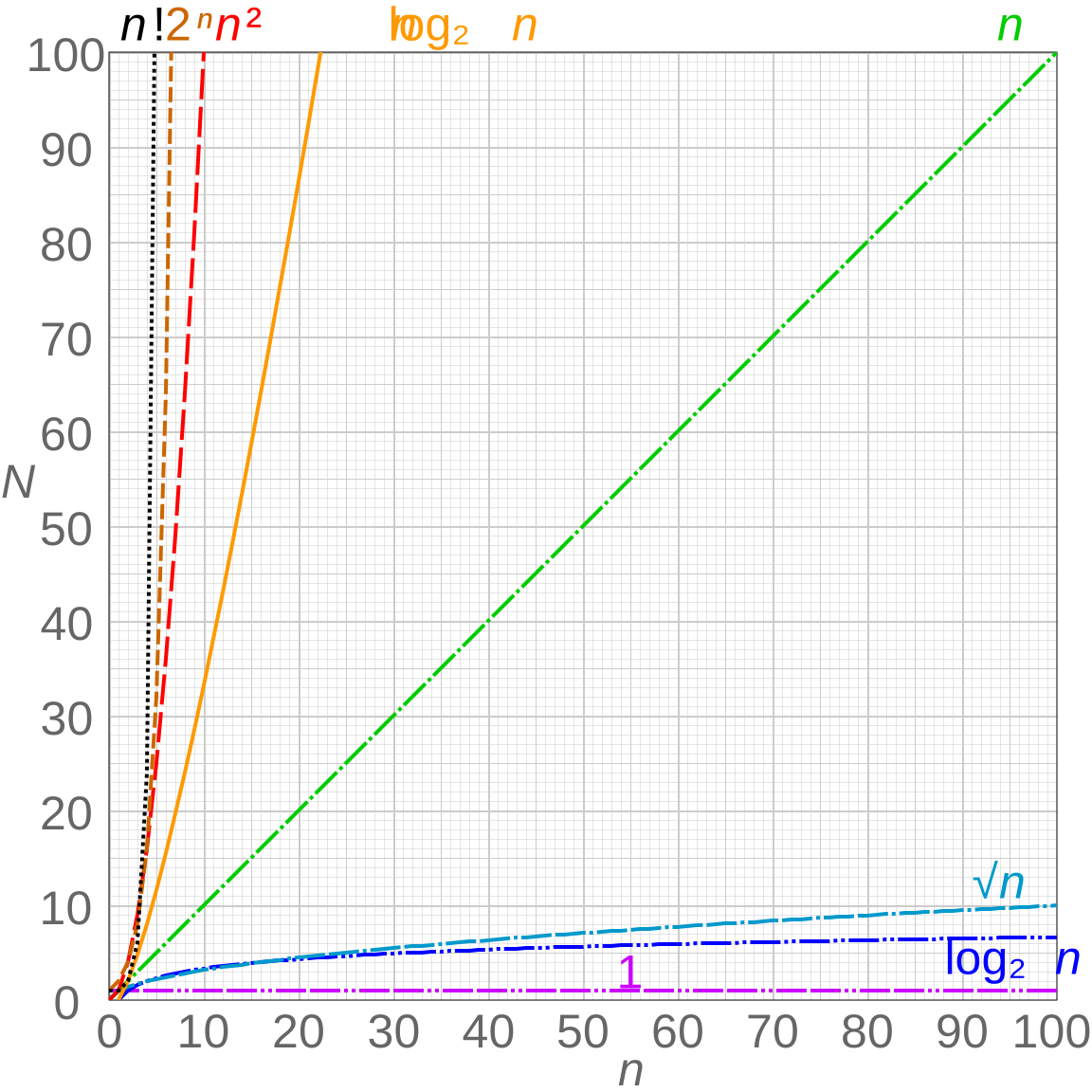
Figure showing the number of operations N as the result of input size n for each function

Complexity Graph

Source: Wikipedia

If we plug in values of n we can see the growth rates

n	10	10²	10³	10⁴	10⁵	10⁶
1	1	1	1	1	1	1
log₂ n	3	7	10	13	17	20
n	10	100	1K	10K	100K	1M
n log₂ n	33	660	10K	133K	1.7M	20M
n²	100	10K	10⁶	10⁸	10¹⁰	10¹²
n³	1K	10⁶	10⁹	10¹²	10¹⁵	10¹⁸
2ⁿ	1K	10³⁰	10³⁰⁰	10^3K	10^30K	10^300K
n!	3.6M	10¹⁵⁷	10^3k	10^35K	10^460K	10^5.6M

Types of measurements

Worst case	Average Case	Best Case
most inefficient input	average input	most efficient input
useful for analysis	provides a realistic view of performance	usually ignored indicated by Omega (Ω) notation

Worst case is the most useful to look at. Some cases the expected average case might be good to look at because it provides a realistic view of perfromance across a range of inputs. The best case is usually ignore but used only to give you give you an overall view of an algorithm.

Examples

O(1) constant time

Input does not affect the run time
Examples:
- Arithmetic Operations
- Comparison Operations (single value)

O(1) constant space

Examples
- Allocating a variable
- Allocating a fixed size array or sorting
  - array with a capacity of 10
  - string with a length of 8 characters

O(log n) logarithmic time

log n is short for log₂ n (based 2 instead of base 10)
Examples
- Binary Search
- Balanced Binary Tree operations
- Heap operations
It is slower than constant time, but faster than linear time

O(log n) logarithmic space

Examples
- Stack space for recursive binary search

O(n) linear time

Examples
- Linear search when you are going through all elements in an array
- Iteration on 1 level

O(n) linear space

Example
- Allocating an array with the length of n
- Allocating a string with the length of n

O(n log n) linearithmic time

Examples
- Quicksort
- Merge sort
- Heap sort
- Fast Fourier transform

O(n²) quadratic time

Examples
Comparison sort
Bubble sort
Nested iteration
Matrix multiplication

O(n³) cubic time

Examples
- Three levels of nested iteration
- 3D matrix storage
- Naive multiplication of two n x n matrices
- Calculating partial correlation

O(2ⁿ) exponential time

Examples
- Towers of Hanoi
- Finding subset of a set
- Combinations
- Recursive fibonacci
- Folding paper example
  - If you had a sheet of paper 0.1mm thickness you only need to fold it 42 times to get to the moon

O(n!) factorial time

Examples
- Traveling salesperson
- Permutations
- Generating anagrams
- Naive sudoku solving

Permutations example

n	1	2	3	4
n!	1	2	6	24
	A	AB BA	ABC ACB BAC BCA CAB CBA

Big O Example

Johann Friedrich Gauss, an 18th Century German Mathematician as a primary school student, was given a task.

Add all the integers from 1 to 100
Standard solution is O(n) where n is 100
Guass' solution is O(1) where n is 100

Measuring complexity

Constant time operations

Arithmetic operations
Comparison operations
Assignment operations
Element access
Print statements

Linear time operations

Iteration of n steps such as an array with size of n

Quadratic / Cubic time operations

Nested iteration, two levels of nesting

Nested operation, three levels of nesting

Big O notation rules

Dropping constants

Allows for simplification
Constants do not significantly impact the growth rate
Allows focusing on inherent efficiency characteristics rather than specific implementation details for ex.
1 for loop, with 1 constant time operation

for i in range(1, n): # O(n)
 print(i)             # O(1) x n
                      # O(n)

1 for loop, with 3 constant time operation

for i in range(1, n): # O(n)
 j = i * 2            # O(1)
 j = j + 1            # O(1)
 print(i, j)          # O(1)
                      # O(1) + O(1) + O(1) = O(3)
                      # O(3) x n
                      # O(3n)

2 for loops, with 1 constant time operation

for i in range(1, n): # O(n)
   j = i * 2          # O(1) x n
                      # O(n)
 
for i in range(1, n): # O(n)
   print(i, j)        # O(1) x n
                      # O(n)
 
                      # O(n) + O(n) = O(2n)
                      # O(2n)

Check for worse case in a minimum constant iteration

from i to min(n, 5): # O(5)
 print(i)            # O(1) x 5
                     # O(5)

Dropping non-dominant terms
- Similar reasons as for dropping constants
- Allows for simplification
- Leaves largest term to dominate as n grows larger (asymptotic analysis)
- Allows non-dominant terms to be removed
  - O(n + 5) = O(n)
  - O(n² + 2n + 1) = O(n²)
  - O(4 + 12n + 12n² + 4n³) = O(4n³) = O(n³)

Different terms for different inputs

Adding complexity for different input sizes, by convention, n is used for a single or first item, m is used for the second item, and so on (p, q, ...)

for i in range(1, n): # O(n)
  j = i * 2           # O(1) x n
                      # O(n)
 
for i in range(1, m): # O(m)
  print(i, j)         # O(1) x m
                      # O(m)
 
                      # O(n) + O(m) = O(n + m)
                      # O(n + m)

Multiple terms for multiple inputs

for i to n:      # O(n)
  for j to m:    # O(m)
    print(i, j)  # O(1)
                 # O(1) x n = O(n)
                 # O(n) x m = O(n x m)
                 # O(nm)